A mean-variance analysis
Context
This page will be a brief summary of the Markowitz mean-variance portfolio analysis I conducted on the below stocks. Feel free to view my code at https://github.com/samperrone25/markowitz-demo.
Data was obtained using pythons yfinance library.
A histogram of Amazon returns were visualised showing a rough normal distribution (no statistical tests were done to verify this).
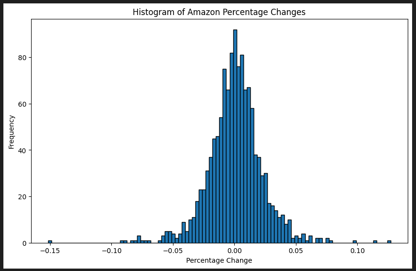
The assumptions of the model, that returns were jointly normally distributed (and so were totally described by their first two moments) and that means, variances and covariances of returns were unchanging during the period of investment were acknowledged.
The problem in Math
A portfolio of up to n risky assets is a vector x of n weights that sum to 1.
Given (n,n) covariance matrix Σ and (n,1) vector of expected returns λ the expected portfolio return is the dot product (*) of λ and x and the variance of the portfolio is the quadratic form x'Σx
Solving for efficient portfolios (a portfolio is efficient if no other has more expected return for the same risk OR less risk for the same expected return) can then be done by minimizing the expression for portfolio variance with constraint x * 1 = 1 and optional constraint x * λ = (a desired level of return).
Monte Carlo simulation of portfolios
Simulating thousands of random portfolio weights and plotting their performance in (expected return, standard deviation (volatility)) space results in:
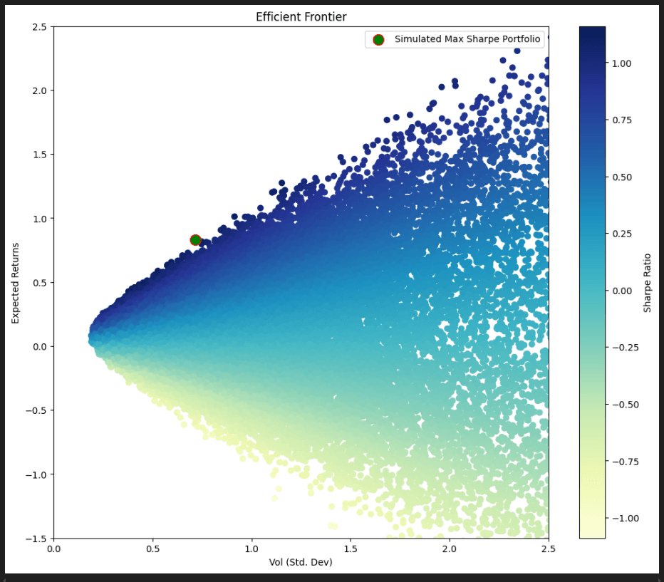
Of interest is the simulated portfolio with the best Sharpe ratio (gradient, or return/risk ratio). This portfolio had the below characteristics, noted here for later comparison with the optimized portfolios.
Optimized Solutions
Scipy optimize.minimize or linear algebra results from [1] [2] were used to find the results in the below table:
As expected the SR of the unconstrained max sharpe portfolio is the highest and the volatility of the global minimum variance portfolio is the lowest. The simulated best sharpe portfolio also got somewhat close to the true best.
The above data was then plotted with the efficient and inefficient frontiers found by minimizing variance while varying the value of the expected portfolio return constraint.

Comparing weights
The weights for the best simulated and optimized portfolios without or with shorts are below
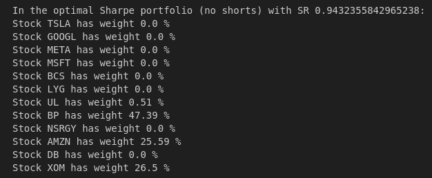
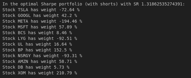
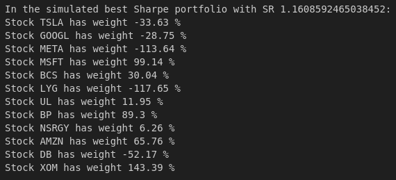
With no short positions it appears that only 4 assets are worth investing when optimizing Sharpe. Also, the Monte Carlo (n=100,000) best Sharpe portfolio weights don't match the best Sharpe weights too closely which isn't surprising given the number of weight combinations it has to search through.
A risk-free rate
A risk free asset yielding 3.5% was introduced and a tangency portfolio was calculated with the below characteristics:
The capital market line (CML) connects the points representing the risk free rate and the tangency portfolio and is visible in the above image in red. Note that it represents a linear combination of the risk free asset and the tangency portfolio and allows us to unlock (expected return, volatility) pairs that weren't possible prior to the risk free assets introduction.
Resources
